import os, sys
sys.path.insert(0, os.path.abspath('..'))  # book root
from calcplot.plots import *

Motivation¶

Examples¶

Example: Area of a Rectangle¶

The formula we’ve all learned for a rectangle is that the area is equal to the length of the base times the height:

A = l\cdot w.

(1)

We need to develop a general framework for working with areas, and we’ll take this as a starting point. As an example, let’s say the length is 5 and the height is 3. We can model this using the function $f(x)=3$ :

plot_integral("$f(x)=3$", f=lambda x: 3+x*10**-26, xlim=(-1, 6), ylim=(-1, 4), a=0, b=5)

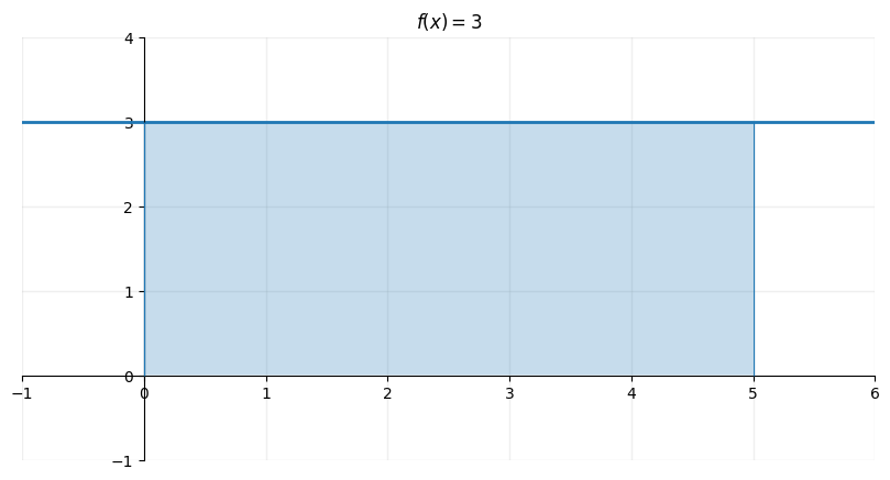
Now we can say that the area of the rectangle is the area between the curve $y=f(x)$ , the $x$ -axis, $x=0$ and $x=5$ .

In general, this means that our area function should have the property that for any constant $h$ ,

A(h, a, b)=h\cdot(b-a).

(2)

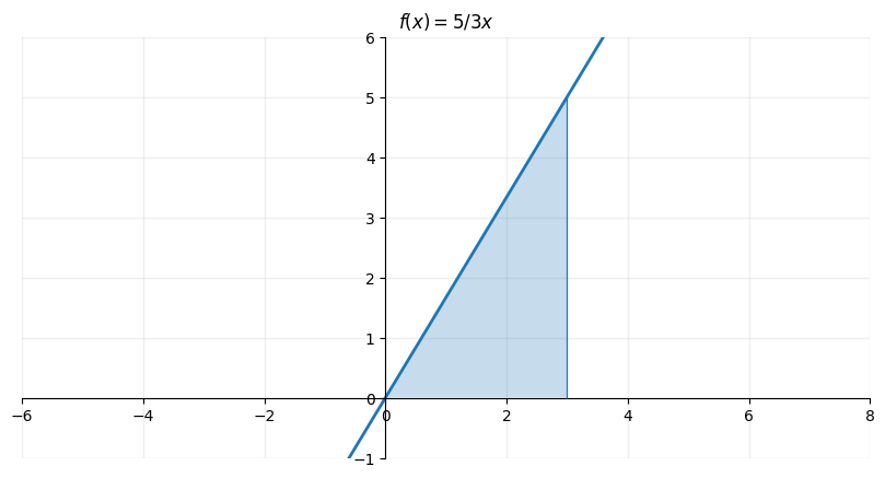
Example: Triangles¶

We also know how to find the area of triangles: $A=\frac{1}{2}b\cdot h$ . For simplicity, let’s stick with right triangles--any triangle can be broken up into right triangles. To model the triangle we can use

f(x)=\frac{h}{b}\cdot x

(3)

. For instance, if we take $h=5$ and $b=3$ , we have

plot_integral("$f(x)= 5/3 x$", lambda x: 5/3*x, (-6, 8), (-1, 6), 0, 3)

Example: Trapezoids¶

We also know how to find the area of trapezoids: $A=\frac{1}{2}b\cdot h$ . For simplicity, let’s stick with right trapezoids--any trapezoid can be broken up into right trapezoids. To model the trapezoid we can use

f(x)=\frac{h}{b}\cdot x

(4)

. For instance, if we take $h=5$ and $b=3$ , we have

plot_integral("$f(x)= 5/3 x$", lambda x: 5/3*x, (-6, 8), (-1, 6), 1, 3)

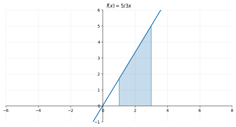
from this, we deduce the property that

A\left( \frac{h}{b}\cdot x, a, b\right) = \frac{h}{b}\cdot \left(\frac{b^2}{2} - \frac{a^2}{2}\right).

(5)

Quadratics¶

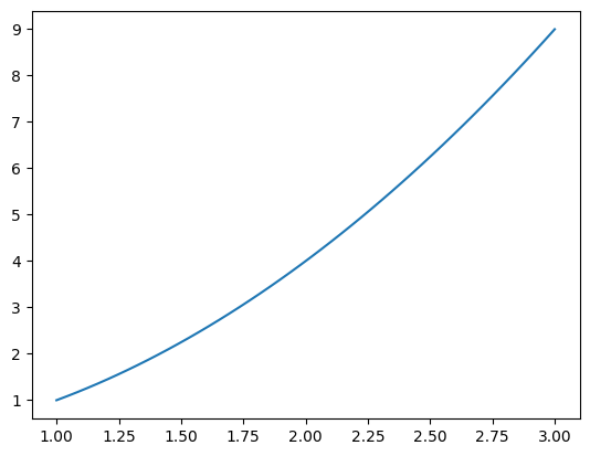
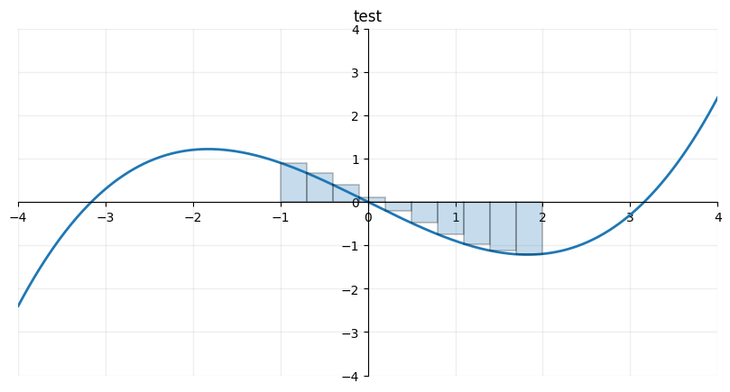
What about something a little more interesting though?

# Example 1: area under a curve
f = lambda x: x**2
xlim=(-1, 3)
ylim=(-1, 5)
a=0
b=2
plot_integral(
title="Area under $f(x)=x^2$ on [-1, 2]",
f=f,
xlim=xlim,ylim=ylim,a=a,b=b)

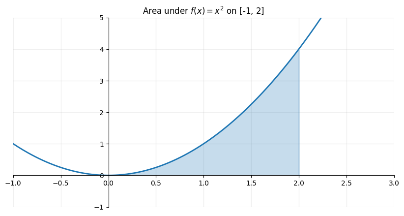
Basic geometry can’t help us with something which curves all the time like this. Let’s see how far we can get though with some basic geometry.

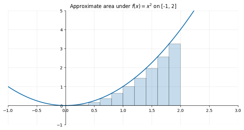
plot_riemann_sum("Approximate area under $f(x)=x^2$ on [-1, 2]", f, xlim, ylim, a, b, 10)

We can approximate the area using rectangles like above.

A(f, a, b)\approx \sum_{i=0}^{n-1} f\left( \frac{b-a}{n}\cdot i + a\right)\cdot \frac{b-a}{n}

(6)

a = 0; b = 2
f = lambda x: x**2
for number_of_rectangles in [2, 10, 100, 1_000, 100_000, 10**6]:
    approximation = sum( f( (b-a)/number_of_rectangles * i + a  )*(b-a)/number_of_rectangles
        for i in range(number_of_rectangles) 
            )
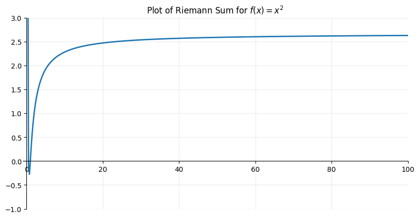
    print(f"N: {number_of_rectangles:,}, approximation: {approximation}")

N: 2, approximation: 1.0
N: 10, approximation: 2.2800000000000007
N: 100, approximation: 2.626800000000001
N: 1,000, approximation: 2.6626680000000027
N: 100,000, approximation: 2.6666266667999796

N: 1,000,000, approximation: 2.66666266666797

It seems like we’re getting close to $2.\overline{6}=\frac{8}{3}$ . Let’s see how far we can get algrebraically.

\begin{align*} A(x^2, a, b) &\approx \frac{b-a}{n}\sum_{i=0}^{n-1}\left(\frac{b-a}{n}\cdot i + a\right)^2,\\ &=\frac{b-a}{n}\sum_{i=0}^{n-1}\sum_{d=0}^2\binom{n}{d}\left(\frac{b-a}{n}\cdot i\right)^d\cdot a^{n-d},\\ &=\frac{b-a}{n}\sum_{d=0}^2\binom{n}{d}\left(\frac{b-a}{n}\right)^da^{n-d}\sum_{i=0}^{n-1}i^d,\\ &=\sum_{d=0}^2\binom{2}{d}\left(\frac{b-a}{n}\right)^{d+1}a^{2-d}S_d(n-1).\\ \end{align*}

(7)

import math
s_0 = lambda n: n
s_1 = lambda n: 1/2 * n**2 + 1/2 * n
s_2 = lambda n: 1/3*n**3+1/2*n**2+1/6*n
plot_function_with_axes(
"Plot of Riemann Sum for $f(x)=x^2$",
lambda n: math.comb(2,0)*( (b-a)/n )*a**2*s_0(n-1)+
math.comb(2,1)*( (b-a)/n )**2*a**1*s_1(n-1)+
math.comb(2,2)*( (b-a)/n )**3*a**0*s_2(n-1)
,
(-1,100),
(-1,3)
)

# Example 1: area under a curve
f = lambda x: 0.1*x**3 - x
xlim=(-4, 4)
ylim=(-4, 4)
a=-1
b=2
plot_integral(
title="Area under $f(x)=0.1x^3 - x$ on [-1, 2]",
f=f,
xlim=xlim,ylim=ylim,a=a,b=b)
plot_riemann_sum("test", f, xlim, ylim, a, b, 10)

# Example 2: midpoint Riemann sum
g = lambda x: np.sin(x) + 1.2
fig2, ax2 = plt.subplots(figsize=(6, 4))
setup_calc_axes(ax2, xlim=(0, 2*np.pi), ylim=(-0.5, 2.5))
plot_function(ax2, g, xlim=(0, 2*np.pi), linewidth=2)
draw_riemann_rectangles(ax2, g, a=0, b=2*np.pi, n=10, method='midpoint', facealpha=0.25)
ax2.set_title("Midpoint Riemann sum for $g(x)=\\sin x + 1.2$ on [0, 2π]")

plt.show()

# assuming you have setup_calc_axes(...) from earlier
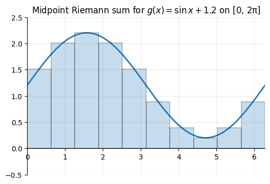
g = lambda x: np.sin(x) + 0.8

fig, ax = plt.subplots(figsize=(6,4))
setup_calc_axes(ax, xlim=(0, 2*np.pi), ylim=(-0.8, 2.2))
S = plot_riemann_with_error(
    ax, g, a=0, b=2*np.pi, n=10, method='midpoint',
    rect_face='none', rect_edge='k', rect_lw=1.2,
    error_color='red', error_alpha=0.35, curve_first=False
)
ax.set_title("Riemann sum with error regions (midpoint rule, n=10)")
plt.show()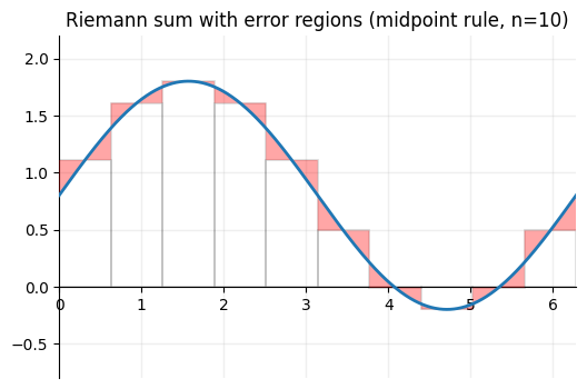

a = 1
b = 3
xs = np.linspace(a, b, 50)
def f(x):
    return x**2

plt.plot(xs, [x**2 for x in xs]);

Integrals

Index

Integrals

Defining the Definite Integral